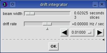
beam width
This sets the integration time which is the size of the sliding window to be averaged.  Units are the number of seconds to be integrated which, in conjunction with an optimal overlap, corresponds directly to the number  of FFT slices. Non coherent integration reduces the variance of the noise  floor by roughly 1/sqrt(2) dB for each doubling of time.  This smooths the spectral randomness which is good for pulling signals out of the noise, but it also has the effect of blurring any non stationary signals, so the correct setting depends highly on signal type and usage.  This control can also be used in an anti-alias fashion on the spectrogram display when the time axis zoom is high.  To make fine adjustments, use the left and right arrow keys on the keyboard.  Note that the beam width control only has an effect on the Spectrogram window since the Average window is an accumulated summation by definition.

drift rate
Also popularly known as "de-chirping", the drift rate slider control compensates for any linear motion in the frequency axis.  Such motion could be caused by the Doppler effect due to the constant angular velocity of the Earth's rotation (about + and - 0.16 Hz / second), or it could be caused by oscillator instability in a tuner circuit, or it could just be the way the signal was constructed.  In any case, correcting for frequency drift prior to integration will increase the effective SNR which is good for weak signal detection.  Clicking on the small arrow in the middle will reset the drift rate to zero.  The left and right arrow keys on the keyboard can be used to make finer adjustments than are possible with the slider, but this method of control is still crude (see the stepping gadget below).

stepping gadget
This is a convenience gadget that modifies the above mentioned drift rate.  Select a "Hz / sec" step size from the option menu and then use the left and right arrows to decrement or increment the drift rate.  Increment values range from 0.00001 to 5.00000 Hz/sec.  This gadget is useful for entering a precise drift rate or for quickly and methodically scanning a range of drift rates.

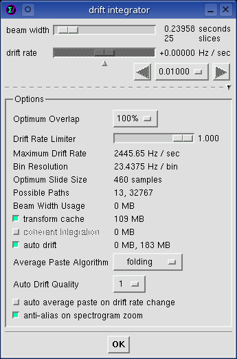
popdown arrow
Clicking the side arrow pops up and down the hidden options box below.  Many drift integrator internal parameter measurements and controls reside here.  Look at this image to see the top section and options box combined.

Optimum Overlap
The effect of this setting is global.  It controls the sliding overlap value that is used by the Average collection, Spectrogram integration, and the Equalization auto collection features.  The default value is 100% which is considered optimal. 

Values less than 100% are speed optimizations which reduce the number of calculations in a beam width integration.  For accuracy, having the optimal overlap set to 100% is best.  For speed, the 50%, 33%, and 25% settings can result in speed ups on the order of 2, 3, and 4 times.  Caution should be exercised because using a less than optimal overlap setting can reduce SNR and in rare circumstances eliminate the signal entirely.  For example, the loss in using the 25% optimal setting is acceptable for equalization since only a rough approximation of the channel shape is required. 

Values greater than 100% are accuracy optimizations.  The 200%, 300%, and 400% settings perform 2, 3, and 4 times the number of slice calculations.   The accuracy increase will be small and slightly measurable.  For general usage the 100% is a very good and "optimal" compromise.  The primary advantage to using an optimal overlap greater than 100% is an increase in the effective maximum drift rate.  For example; a 200% optimal overlap will have twice the maximum drift rate.

The off option disables the optimum overlap calculation and uses the slide size value that is defined in the Scroll Control window.  This option is particularly useful when integrating Correlation and Raster transforms since it retains the line width alignment.

Note that changing the optimal overlap will have an effect on the memory usage of the transform cache, maximum drift rate, and the computational speed.

Drift Rate Limiter
This limiter ranges from 0.001 to 1.000 and is a multiplier that operates on the maximum drift rate.  When moving this slider notice the effect on the Maximum Drift Rate and the Possible Paths values.  A 1.000 setting chooses the highest maximum drift rate allowed while a smaller value artificially reduces it.  For auto drift operation, limiting the maximum drift rate is a way to reduce memory and CPU usage.  It also reduces extraneous hits that are above the rate limit.  For non auto drift operation this slider controls the stepping click range and the range of the drift rate slider.

Maximum Drift Rate
This line displays the maximum linear drift rate value which can be thought of as a frequency velocity, it has units of Hz per second.  The maximum drift rate defines the search domain limits from negative to zero (stationary) to positive {-0.17160 ... +0.17160}.  In certain circumstances (folding algorithm with a quality of 2+) two comma separated maximum drift rate values will be displayed, in this case the leftmost value applies to the spectrogram display and the rightmost value applies only to the Average Paste operation.

Bin Resolution
On the frequency axis, each FFT bin corresponds to this amount of Hz.  Changing the FFT size and the sample rate change this value.  The larger the bin resolution the larger the maximum drift rate will be.

Optimum Slide Size
This is a function of FFT size and the optimum overlap value.  It is the amount of samples that each slices is incremented while performing drift integration.

Possible Paths
Each path can be thought of as a distinct and unique drift rate within the domain limit defined by the maximum drift rate.  When auto drift is disabled one possible path value for both the Spectrogram and the Average Windows is displayed which represents the number of mouse clicks of the stepping gadget that are required to go from the negative to the positive maximum drift rate.  When auto drift is enabled there are two comma separated possible paths, the left value is for the spectrogram display while the right value is for the Average Window (either paste or record).  The number of possible paths is a function of many parameters which include time duration (beam width and selection size).  More paths means better rate accuracy and fuller coverage.

Beam Width Usage
The amount of memory buffers (in megabytes) used by the beam width.

transform cache
The transform cache remembers past calculations for the purpose of speeding up future redundant calculations.  Most operations that redraw the spectro window will benefit such as changing beam slices, drift rate, Hz scroll bar position or zoom, color aperture, transform space, and channel color.  Other operations such as average pastes and auto equalization will also be sped up.  The transform cache is most effective when a large FFT size is chosen because large FFT's are slow.  The speed increase can be dramatic.  For example; with a 32768 point FFT size, an average paste operation that used to take 30 seconds now requires less than 1 second to complete.  This allows the user to modify variables such as drift rate and beam width and get near real-time performance.  It makes searching a large variable space very fast.  It also makes moving the Hz scrollbar a pleasant and usable option when very large FFT's are used.

The downside to the transform cache is that it can use a very large amount of memory.  With more than a gigabyte of RAM in certain extreme cases, swap thrashing can result, so caution is advised.  To the right of the transform cache option button is the memory usage estimate (in megabytes) which changes dynamically as other baudline options are modified.

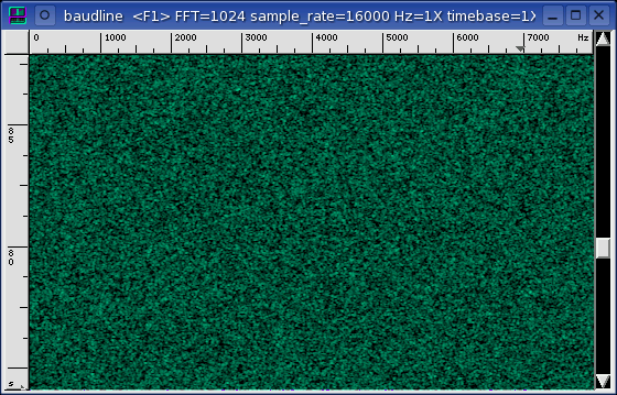
auto drift
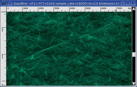
The two pictures above demonstrate the auto drift feature automatically pulling a weak non-linear drifting signal out of the noise.  The first image has the auto drift feature disabled and the spectrogram looks like white Gaussian noise.  The second image has auto drift enabled and a sine frequency modulated carrier shape is clearly visible.  This is the power of auto drift.

Auto drift is an algorithm that searches all of the possible linear drifting paths for the correct solution.  It is an automatic procedure that scans from the negative maximum drift rate to the positive maximum drift rate while searching each and every frequency bin for the strongest drift rate solution.  This is similar to manually clicking the stepping gadget through every possible path while keeping track of the slopes of the moving peaks.  Depending on the specific settings, this can result in thousands of unique paths and billions of distinct drift vectors.  The auto drift algorithms are extremely efficient yet the shear volume of drift vectors makes this is a very CPU intensive operation.

The auto drift algorithm is designed to track constant linear drifts.  This can be restated as "straight lines sum up nicely."  The FM sine in the above spectrogram image is actually non-linear in that the acceleration is not constant.  Since it is difficult to build a clean sine wave from straight lines the FM sine shape is the worst possible test signal from the auto drift point of view.  Yet, as suboptimal as it is, auto drift can track the FM sine with great clarity (see the above spectrogram).

Auto drift isn't actually a single algorithm but it is a collection three different algorithms all of order O(n * log n).  Three algorithms that perform the same auto drift concept on the Spectrogram display, the Average Paste operation, and the Average record collect.  Baudline can analyze data files in batch mode or in real-time and view the solutions in the Average spectrum display or see the spatial time variations in the graphical Spectrogram display.  This flexibility empowers the user with extra linear-drifting weak-signal sensitivity in all of baudline's frequency displays and modes of operation. 

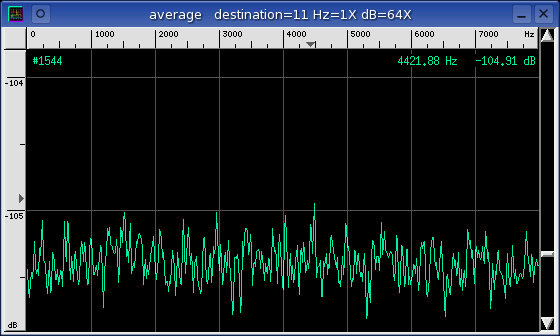
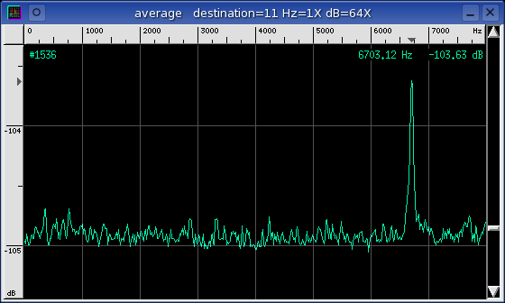
The two Average spectrum plots below demonstrate auto drift's ability to extract a weak linear sweep from a strong noise floor.  The auto drift feature is disabled in the first spectral plot and it is enabled in the second spectrum plot for a before-and-after effect.  What initially looks like noise in fact has a drifting tone embedded in it (a 6703 Hz peak that is about 7 sigma above the noise floor).  The Average collect durations (#) are the same for both spectral plots yet the auto drift enabled one has about half the variance.  Also of interest is that the mean noise floor is about half a dB higher for the auto drift case.  Both of these spectral observations can be explained by how the fundamental auto drift mechanism works.  Thousands of unique drift vectors are being summed in the search for the ideal solution.  More vectors means a lower variance.  More potential solutions translates into a slightly higher noise floor.

This may seem similar to those of you familiar with the seti@home project or the Targeted Search System (TSS) used by the Project Phoenix.  Indeed it is.  Besides improved flexibility, speed, and sensitivity, a key difference that sets baudline apart is the Spectrogram auto drift view.  This is a truly innovative display that allows the user to visualize drifting signals in a manner never before possible.

To the right of the toggle button and the auto drift label are two comma separated megabyte (MB) buffer allocation estimates.  The left value is the amount of memory needed for the Spectrogram auto drift operation.  The right value is the Average auto drift buffers estimate for either the Paste (pause) or Record operation.  Caution should be observed since a folding Average paste operation can consume more than a gigabyte of RAM with large data sets, this can lead to swapping and reduced system performance.

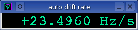The values of the internal drift vectors can be queried with the auto drift rate measurement window.  The units are in Hz/second.  Note that the measurement granularity is a function of algorithm type and the number of possible paths (see auto drift quality parameter).  The auto drift measurement display can be configured to track the main fundamental, the mouse position, or be range bounded.

Possible uses of the auto drift feature are any disciplines with signal sources that experience strong Doppler shift such as astrophysics (radio astronomy), satellite telemetry, SETI, sonar, and Gravitational Wave detector physics.  Another novel use is tracking a wandering tone that is buried deep in the noise.  If you find an interesting use for auto drift please let us know, we would be interested in hearing about it.

Average Paste Algorithm
This option selects which auto drift algorithm to use when an Average Paste operation is performed.  There are two classes of algorithm: an all paths search and a folding search.  Each has its advantages and limitations.

The O(n^2) algorithm is a very slow all paths search and it should never be used except for comparison purposes.  The running sum algorithm is of the all-paths-search class but it is almost an order of magnitude faster than O(n^2) due to sweep redundancy optimizations.  The accuracy of running sum is practically the same as the O(n^2) algorithm.

The folding algorithm is a fast O(n * log n) approximation that is a good choice for general auto drift work.  The double stuff algorithm is a higher quality variation of the of the folding class with twice the path resolution and half the maximum drift rate.  It is an excellent choice if the lower maximum drift rate and higher (double) memory and CPU usage is tolerable. 

The folding algorithm is by far the quickest being about 10X faster than running sum which is in turn about 10X faster than O(n^2).  The down side is that the folding algorithm is an approximation and it does have measurable error.  The double stuff algorithm is probably the best compromise, it is an excellent balance of speed and accuracy, but this of course depends on your particular mission parameters.

Pressing Alt+D in the Average window will transfer the auto drift rate value of the bin under the mouse to the drift rate slider in the Drift Integrator window.  Doing this while auto drift is disabled will allow different drift rates to be quickly auditioned and displayed.  Note that this bin value can also be monitored with the auto drift rate measurement window.

Auto Drift Quality
This is a sensitivity control that allows the user to modify the number of possible paths.  More paths equates to a higher quality and more accurate calculation.  The quality value is selectable from 1 (the lowest) to 10 (the highest).  It controls all 3 operational modes of the auto drift function (spectrogram, average paste, and average record).  The default quality value is 1 which is the fastest and uses the least memory.  Each step increase of the quality doubles the number of paths which will roughly double both memory and CPU usage.  If your hardware is capable enough then a quality setting of 2 or 3 will give a mild improvement.  Quality values of 4+ use excessive hardware resources and are generally not recommended.  With folding class paste algorithms changing the quality will also change the Maximum Drift Rate.  When changing quality values note the effect on the possible paths and the auto drift memory usage.  Using too much memory will cause severe swapping.

auto average paste on drift rate change
This feature makes scanning through a range of drift rates while analyzing the average spectral domain a simple one click operation.  Whenever the drift rate changes, an automatic paste into the Average window is triggered.  This is equivalent to choosing the Paste option in the Average window's Collect menu.  It will either be a paste of the currently selected data or a paste of all data if nothing is selected.  This feature is only active when in the pause mode, when the transform cache is enabled, and when auto drift is disabled.

anti-alias on spectrogram zoom
As the spectrogram time axis is zoomed in or out this option automatically sets the beam width slider to an optimal value such that all sample data is transformed and averaged.  Like anti-alias decimating in the input devices window, this option is like performing anti-alias filtering in the spectrogram time domain.  The effect is like smoothing and it provides a more accurate view of the spectrogram display.  This function is particularly useful when looking for small transients in a very large data file.