baudline solution - sample rate stability

Abstract

Sample rate stability
E. Olson, Aug 16 2005

A calibrated and stable time source is critical for accurate DSP. Differences in audio clock circuitry, thermal drift, and NTP latency can all affect the sample rate which will lead to time / frequency measurement errors. This app note will develop a method for measuring, calibrating, and tracking sample rate errors with the baudline signal analyzer.

Internal Calibration

Various sample rates can be monitored and calibrated with the Input Device and the Output Device windows. This feature utilizes a tight coupling between the system clock and the audio driver which allows the absolute sample rate to be measured. Operation is simple and it is designed for general purpose use. No external hardware or wiring is required and it works during record and/or playback modes. See the Input Devices image below:

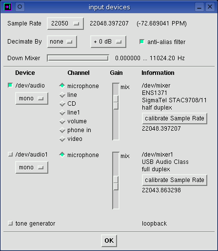
The general idea is to set the sample rate, calibrate baudline, and then make a measurement. A correction factor is only valid for a particular sample rate. So changing the sample rate requires a recalibration. Here is how this feature is used:

procedure

Setup baudline mission parameters. (open windows, adjust controls, ...)
Put baudline into record or play mode.
Watch the sample rate estimate converge in the Input and Output Device windows.
Wait from one minute to an hour or more depending on desired accuracy. Baudline can be used during this time.
After the sample rate estimate has stabilized to an acceptable level of precision hit the calibrate button.
Note the new rate and PPM measurement display next to the Sample Rate option menu.
While using baudline, periodically check that the current sample rate estimate has not diverged significantly from the calibrated rate. If it has then recalibrate.
Note that pausing baudline resets the sample rate estimate convergence.

The plot below demonstrates how the sample rate estimate converges with a reducing variance as the collection time increases. The data for the convergence plot was captured with the -debugrate command line option.

convergence speed
Latency controls the variance and the convergence speed of the sample rate estimate. System load and kernel options such as real-time preemption can play a major role. So can kernel type; for example the FreeBSD kernel has a significantly different variance signature than the Linux kernel due to different scheduling algorithms and internal coding latencies.

The calibration convergence speed can be improved by reducing baudline's audio fragment latency. A smaller fragment size means less latency. Try changing the fragment size parameter to values of 6, 7, 8, or 9. For example:

baudline -fragsize 6

External Calibration

An external reference quality tone generator can be used for a higher performance sample rate calibration. Special hardware and some extra wiring are required but the accuracy and convergence speed should be dramatically improved with this method.

procedure

Start baudline, choose a sample rate, and begin capture.
Attach an external tone generator and dial in a test frequency that is within the Nyquist band. This is the "input" rate.
Open a Hz measurement window and increase the number of precision digits and the record averaging slices. This is the "measured" rate.
Calculate the PPM error and then restart baudline with this calibrated value:
- ppm = (input rate / measured rate - 1.) * 1000000.
- baudline -calibratesr 123.4567
For a sanity check compare this PPM value with that calculated by the Internal Calibration technique mentioned above.

Full Duplex

It is important to check the relationship between the input and output sample rates when operating in the full duplex mode. If the ADC and the DAC clocks are locked together then the input and output sample rates should be equal. If the ADC and DAC each have their own clock then the relationship is floating. Or there may be unusual clock divider circuitry at specific sample rates. The number of possible clock synthesis designs are many. So it is always a good idea to test this synchronization. Fortunately there are two easy techniques for performing this with baudline.

The Internal Calibration method can be used when running baudline in the full duplex mode and it is a valuable tool for determining the absolute sample rates of both channels. If they are equal then the ADC and DAC clocks are locked and all is good. A significant difference means that the clocks are not 1:1 locked and full duplex sample rate calibration is not possible. By comparing the input and output sample rates a relative PPM error can be calculated.

loopback
Another technique for determining the ADC and DAC clock relationship is the the full duplex Tone Generator loopback method. It is a relative measurement of the PPM error between the full duplex input and output channels that is very accurate. The idea is to create a test signal, loop it back, and measure how much the frequency changes. Baudline's Tone Generator window is used to create a clean sine wave test signal. The analog signal source is then looped back to the input channel with an external loopback cable or with the internal "volume" mixer option and then recorded. For best results the signal level should be strong without any distortion but high SNR is not as critical here as it is with other types of tests.

The frequency of the sine wave is then measured to several decimal places of accuracy with the Hz measurement window. The digital tone generator loopback option in the Input Devices window can be used to allow both the input and output frequency to be measured and displayed in the same window. Like in the previous Internal Calibration method, if the input and output frequencies are the same then the ADC and DAC clocks are locked. A significant difference means clock mismatch. The frequency difference between the input and output channel be calculated as a PPM error.

Both of the above methods can be used at the same time and their results should be equivalent. The loopback method is faster and is more accurate but it is actually a good idea to perform both and compare. Here is a review of the three possible input / output clock outcomes:

1.0 ratio - ADC and DAC clocks locked
fractional relationship - integer frequency divider at work
floating relationship - separate ADC and DAC clocks

A fractional or floating clock relationship means that accurate full duplex sample rate calibration is not possible with that particular audio card.

ENS1371 Test

The full duplex methods described above were performed on an Ensoniq AudioPCI ENS1371 audio card that has a SigmaTel STAC97 codec. The ES1371 card is also known as the Sound Blaster PCI16, PCI64, or the SB128. It is a low cost audio card of moderate performance that has a very interesting full duplex characteristic.

absolute
The input and output sample rates were estimated with the Internal Calibration method. The convergence plot below was created with with the -debugrate command line option and two distinct sample rates are visible.

The "input" curve represents the ADC clock and the "output" curve represents the DAC clock. The difference between the input and output sample rate is about one sample per second. This test was conducted at all of the standard sample rates and the results are in the table below:

`sample rate`	`input rate`	`output rate`	`input error`	`output error`
`5510`	`5510.01525`	`5510.01997`	`+2.7677 PPM`	`+3.6243 PPM`
`8000`	`8000.01144`	`8000.01144`	`+1.4300 PPM`	`+1.4300 PPM`
`11025`	`11025.0543`	`11024.9870`	`+4.9252 PPM`	`-1.1791 PPM`
`12000`	`11999.9420`	`11999.9420`	`-4.8333 PPM`	`-4.8333 PPM`
`16000`	`16000.0097`	`16000.0097`	`+0.6062 PPM`	`+0.6062 PPM`
`22050`	`22050.2609`	`22050.0624`	`+11.8322 PPM`	`+2.8299 PPM`
`24000`	`24000.0365`	`24000.0365`	`+1.5208 PPM`	`+1.5208 PPM`
`32000`	`32000.0607`	`32000.0302`	`+1.8969 PPM`	`+0.9438 PPM`
`44100`	`44101.0821`	`44100.0672`	`+24.5374 PPM`	`+1.5238 PPM`
`48000`	`48000.1027`	`48000.1027`	`+2.1396 PPM`	`+2.1396 PPM`

The output error is less than 5 PPM for all of the sample rates, and it is less than half that for the majority of them. The input error is also less than 5 PPM for all of the sample rates except 22050 and 44100. This discrepancy highlights that something unusual inside the ENS1371 is going on at those two rates.

Mainstream audio cards typically have sample rate errors in the 50 to 100 PPM range. The clocks on standard PC's usually have an error of 40+ PPM. So in retrospect, the ENS1371's median error of 5 PPM is quite good.

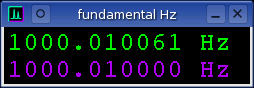
relative

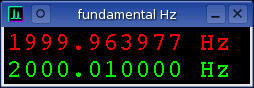Next, the full duplex loopback method is used to measure the relative difference between the input and output channels. A 2000.01 Hz sine wave is the test signal. The green channel is the digital loopback from the Tone Generator output and the red channel is the analog loopback from the ENS1371 recorded input. Six decimal places of frequency resolution accuracy are displayed in the fundamental Hz measurement window. The Average window below is another way of visualizing this error. The frequency axis has been zoomed way in and the two distinct spectral peaks are visible.

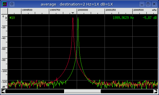
Both of these techniques are measuring the same phenomena which expose that some sort of integer frequency divider is at work. Through careful measurement the internal circuitry design details are being uncovered. Below is a table of the measurements and calculated PPM errors for all of the standard sample rates. The "rate" columns utilize the Internal Calibration fragment method and the "Hz" columns use the tone loopback method. The PPM error columns compare their respective input and output values. The rate_error column should be equal to the Hz_error column since they are different methods of measuring the same thing.

`rate in`	`rate out`	`rate error`	`generate Hz`	`record Hz`	`Hz error`
`5510.01525`	`5510.01997`	`-0.8566 PPM`	`1000.010002`	`1000.010859`	`-0.8570 PPM`
`8000.01144`	`8000.01144`	`+0.0000 PPM`	`2000.010000`	`2000.010000`	`+0.0000 PPM`
`11025.0543`	`11024.9870`	`+6.1043 PPM`	`2000.010000`	`1999.997730`	`+6.1350 PPM`
`11999.9420`	`11999.9420`	`+0.0000 PPM`	`2000.010000`	`2000.010000`	`+0.0000 PPM`
`16000.0097`	`16000.0097`	`+0.0000 PPM`	`2000.010000`	`2000.010000`	`+0.0000 PPM`
`22050.2609`	`22050.0624`	`+9.0022 PPM`	`2000.009999`	`1999.992015`	`+8.9920 PPM`
`24000.0365`	`24000.0365`	`+0.0000 PPM`	`2000.009999`	`2000.009999`	`+0.0000 PPM`
`32000.0607`	`32000.0302`	`+0.9531 PPM`	`2000.010000`	`2000.008093`	`+0.9535 PPM`
`44101.0821`	`44100.0672`	`+23.0136 PPM`	`2000.010000`	`1999.963977`	`+23.0119 PPM`
`48000.1027`	`48000.1027`	`+0.0000 PPM`	`2000.010001`	`2000.010001`	`+0.0000 PPM`

validation
The most important observation of this experiment is that the two test techniques produce results that differ by less than 1%. The loopback method has a much faster convergence rate while the Internal Calibration method is a background test that can be conducted while baudline is performing other actions. There are benefits to each method, so depending on mission goals, either testing procedure will produce valid clock synchronization results.

analysis
The second observation is that the ENS1371 card has some very strange clock logic. The sample rates that are integer multiples of 11025 have large PPM errors. This means that the input and the output sample rates differ by a small but fixed amount. For the sample rates { 11025, 22050, 44100 } the i/o PPM error is { 6.135, 9, 23 } which is an unusual progression. The 32000 sample rate is an exception with a +0.9535 PPM. Note that the 5510 sample rate doesn't follow this PPM error trend but 5510 is not exactly half of 11025 so some other mode of divisor operation is at work.

The 48000 to 44100 sample rate conversion is a difficult ratio for polyphase filter generation but this is an unrelated problem since it doesn't explain why the ADC and the DAC clocks would need to be different.

The reason for the clock mismatch at the 11025 rate multiples is unknown. It could be due to either hardware design or the software driver. The ramifications of this are that the sample rate cannot be accurately calibrated when doing full duplex operation on the ENS1371 card at these particular rates. If full duplex frequency accuracy is important then the sample rates with measurable PPM error values should be avoided.

Thermal Drift

Temperature can have a significant impact on clock frequency. This is called thermal drift and it is the reason why Cesium (Cs) and Rubidium (Rb) reference quality clocks are oven regulated. A computer's system (CPU) clock and audio card clock are prone to thermal drift and subject to periodic fluctuations. Below is a sample rate estimate plot that demonstrates a daily 24 hour cycle (1 day = 86400 seconds).

The daily swings shown above equate to an error of about 0.5 PPM. Note that the sample rate estimate plot is an accumulated function. It is an exponential convergence. Variations, fluctuations, and distortions will slowly smooth out over time. It is meant to be an indicator of the average sample rate since the start of the test and not the true instantaneous sample rate.

The sample rate correction factor is stored and it can be used between different baudline sessions. The plot above demonstrates how thermal changes over the course of a day can invalidate a previous correction factor. If ultimate frequency accuracy is required then frequent recalibration is necessary.

Another strategy is to constantly be in a state of calibration. Fortunately baudline makes doing this easy by calculating sample rate estimates whenever baudline is recording or playing. Just keep the Input and/or Output Device windows open and monitor how the sample rate estimate fluctuates. After the convergence period and when the error becomes too large simply press the "calibrate Sample Rate" button.

NTP Distortions

The Network Time Protocol (NTP) is a great way to keep a system's clock synchronized to within a millisecond of standard time. Since computer system clocks typically have an error of about 50 PPM, using NTP corrects this and actually makes baudline's sample rate estimate extremely accurate. Without NTP the sample rate correction wouldn't be any better than the PPM error of the system clock. NTP is a good thing.

Unfortunately the Internet can become congested and network latency can increase dramatically. When this happens the NTP algorithms attempt to correct the situation by stepping and slewing the system clock. This works well when the required clock tweaks are minor but when the corrections become major then some wild behavior erupts.

Delay, offset, and jitter are quality metrics that NTP uses internally for decision making. NTP has a fairly complex state machine that is constantly tracking and correcting. The severity of clock error determines which step and slew algorithm to utilize. The differing algorithmic correction formula generate a colorful array of strange shapes and curves.

The plots below were made with the -debugrate command line option during a time of major Internet congestion.

convex bounces (1 PPM)

quantum steps followed by concave pointy waves (4 PPM)

steep linear slopes with large discontinuities (4 PPM)

Notice how in all three plots the sample rate begins as a constant fairly stable and predictable value. Then the Internet congestion hits and the NTP state machine becomes perturbed. The NTP algorithm then attempts to fix the error which induces a state of chaos. The system then oscillates for several hours. When the network congestion clears the sample rate returns to a stable value almost exactly where it was before it all began.

This demonstrates that the audio card's clock and the system clock are free running and not linked. It is also important to note that baudline's sample rate estimate is an accumulated measurement that damps any movement. If it was an instantaneous measurement then the changes due to the clock adjustments would be much greater. The 4 PPM error in the final image could of been magnified to possibly 400+ PPM under different collection circumstances.

potential solutions
There are a couple possible solutions to this problem. NTP can disabled while testing but the validity of the initial sample rate calibration will need to be verified. Another solution is to have a local NTP stratum 0 time source such as a GPS unit.

It is important to note that the NTP fluctuations only cause an error with the current sample rate estimate that is in progress. Previous estimates are still correct and the sample collection and timing accuracy is not hindered in any way. So the real world effects of these strange NTP shapes is minimal. Still, if the sample rate is calibrated during a congestion burst then that erroneous estimate will be in use until the next calibration. The real danger is in not knowing.

Conclusion

Three different techniques for measuring sample rate clock error have been explored. Two are absolute measurements and are useful for recalibration purposes; the Internal and External methods. Another technique is a relative measurement, the full duplex tone generator loopback method, and it is valuable as a quick and accurate check of the ADC and DAC clock relationships. Each method has unique benefits and is designed for different test situations and requirements.

Both thermal drift and NTP were shown to be sources of sample rate error. So a working routine of constant sample rate monitoring and frequent recalibration is important if accurate frequency measurements are desired.

It was also shown that an audio card's distribution of PPM error does not have to be uniform for all the sample rates. In fact, specific rates on certain cards might be problematic and are best avoided. With these different techniques the inner workings of an audio card's circuitry can be observed through careful measurement.

So, sample rate estimation and calibration can be used for improving the accuracy of frequency measurements and they can also be used as tools for learning more about the inner details of specific hardware.